---
title: "Oncology Survival"
order: 4
---
```{r setup script, include=FALSE, purl=FALSE}
invisible_hook_purl <- function(before, options, ...) {
knitr::hook_purl(before, options, ...)
NULL
}
knitr::knit_hooks$set(purl = invisible_hook_purl)
```
## Introduction
This guide demonstrates how pharmaverse packages, along with tools from the
tidyverse, can be used to create standard oncology efficacy Tables, Listings,
and Graphs (TLGs) using the `{pharmaverseadam}` `ADTTE_ONCO` and `ADRS_ONCO`
datasets as input.
The packages used, with a brief description of their purpose, are as follows:
* [`{pharmaverseadam}`](https://pharmaverse.github.io/pharmaverseadam/): provides
CDISC ADaM example datasets for use in pharmaverse examples and tests.
* [`{ggsurvfit}`](https://www.danieldsjoberg.com/ggsurvfit/): eases the creation
of publication-ready time-to-event (survival) figures built on `{ggplot2}`.
Includes `Surv_CNSR()` to handle CDISC ADTTE censoring conventions natively.
* [`{gtsummary}`](https://www.danieldsjoberg.com/gtsummary/): creates
publication-ready summary and analytical tables. Used here for survival and
tumor response summaries.
* [`{dplyr}`](https://dplyr.tidyverse.org/): provides data manipulation
functions used to prepare and filter the ADaM data.
* [`{forcats}`](https://forcats.tidyverse.org/): provides factor manipulation
utilities used to order RECIST response categories for table display.
* [`{broom}`](https://broom.tidymodels.org/): extracts tidy model output from
Cox regression fits — used to build the subgroup forest plot.
* [`{survival}`](https://cran.r-project.org/package=survival): provides `coxph()`
for fitting Cox proportional hazards models.
The outputs produced in this example are:
1. **Kaplan-Meier plot** with confidence intervals, risk table, and median
guideline — a standard figure for oncology efficacy reporting.
2. **Risk table** displayed beneath the KM plot showing number at risk, events,
and censored counts at each time point.
3. **Median survival table** with 95% confidence interval, suitable for
inclusion in a clinical study report (CSR).
4. **Survival probability table** at selected time points.
5. **Best Overall Response table** with category counts, percentages, and
inline ORR (CR + PR) summary from `ADRS_ONCO`.
6. **Stratified KM plot** using the built-in `ggsurvfit::adtte` four-arm trial
dataset to illustrate multi-arm analyses.
7. **Subgroup forest plot** showing PFS hazard ratios by hormone receptor status
and prior radiotherapy history using `ggsurvfit::adtte`.
---
## Setup
We load the required packages and read `ADTTE_ONCO` and `ADRS_ONCO` from
`{pharmaverseadam}`. `ADTTE_ONCO` is the oncology-specific TTE dataset generated
from the `{admiralonco}` template — it contains three endpoints (OS, PFS, RSD)
with treatment arm variables already merged in. `ADRS_ONCO` is the tumor response
dataset containing per-visit and summary response parameters (BOR, CBOR, RSP)
derived from RECIST 1.1 assessments.
Because the CDISC ADTTE censoring variable `CNSR` is coded `1 = censored /
0 = event` (the reverse of base R's `survival::Surv()` convention), we use
`Surv_CNSR()` from `{ggsurvfit}` throughout to avoid mis-coding errors.
```{r setup}
#| message: false
#| warning: false
library(pharmaverseadam)
library(ggsurvfit)
library(ggplot2)
library(gtsummary)
library(dplyr)
library(forcats)
library(broom)
library(survival)

# ── Read data ──────────────────────────────────────────────────────────────────
adtte_onco <- pharmaverseadam::adtte_onco

# ── ADRS_ONCO: tumor response data ───────────────────────────────────────────
adrs_onco <- pharmaverseadam::adrs_onco |>
  filter(ARMCD != "Scrnfail")

# Overview of available endpoints and their event rates
adtte_onco |>
  group_by(PARAMCD, PARAM) |>
  summarise(
    N           = n(),
    N_events    = sum(CNSR == 0),
    Pct_events  = round(100 * mean(CNSR == 0), 1),
    Median_AVAL = round(median(AVAL), 2),
    .groups     = "drop"
  )
```
> **Why PFS for this example?** OS in early-phase oncology trials typically has
> few events (most subjects are still alive), producing a near-flat KM curve
> with a median that cannot be estimated — not ideal for illustration. PFS has
> more events and a shorter follow-up window, giving a more informative curve.
> The code below uses `PARAMCD == "PFS"`; swap to `"OS"` or `"RSD"` as needed.
> Note that `{admiralonco}` uses `"RSD"` (not `"DOR"`) for Duration of Response.
::: {.callout-note}
`pharmaverseadam::adtte_onco` is a small example dataset with limited events
across all endpoints, so the resulting KM curves and tables are for illustration
only and should not be interpreted clinically. For a richer example with more
events and better-separated arms, see the
[Stratified KM Plot](#stratified-km-plot-ggsurvfitadtte) section below, which
uses the `ggsurvfit::adtte` four-arm breast cancer trial dataset.
:::
```{r filter-pfs}
#| message: false
#| warning: false
# ── PFS endpoint ────────────────────────────────────
adtte_pfs <- adtte_onco |>
  filter(PARAMCD == "PFS")

# Preview key variables
adtte_pfs |>
  select(USUBJID, PARAM, PARAMCD, AVAL, CNSR, EVNTDESC, CNSDTDSC) |>
  head(5)
```
> **Note on CNSR coding:** In CDISC ADTTE, `CNSR = 0` indicates an **event**
> and `CNSR = 1` indicates **censoring**. `Surv_CNSR(AVAL, CNSR)` handles this
> correctly without requiring manual recoding.
---
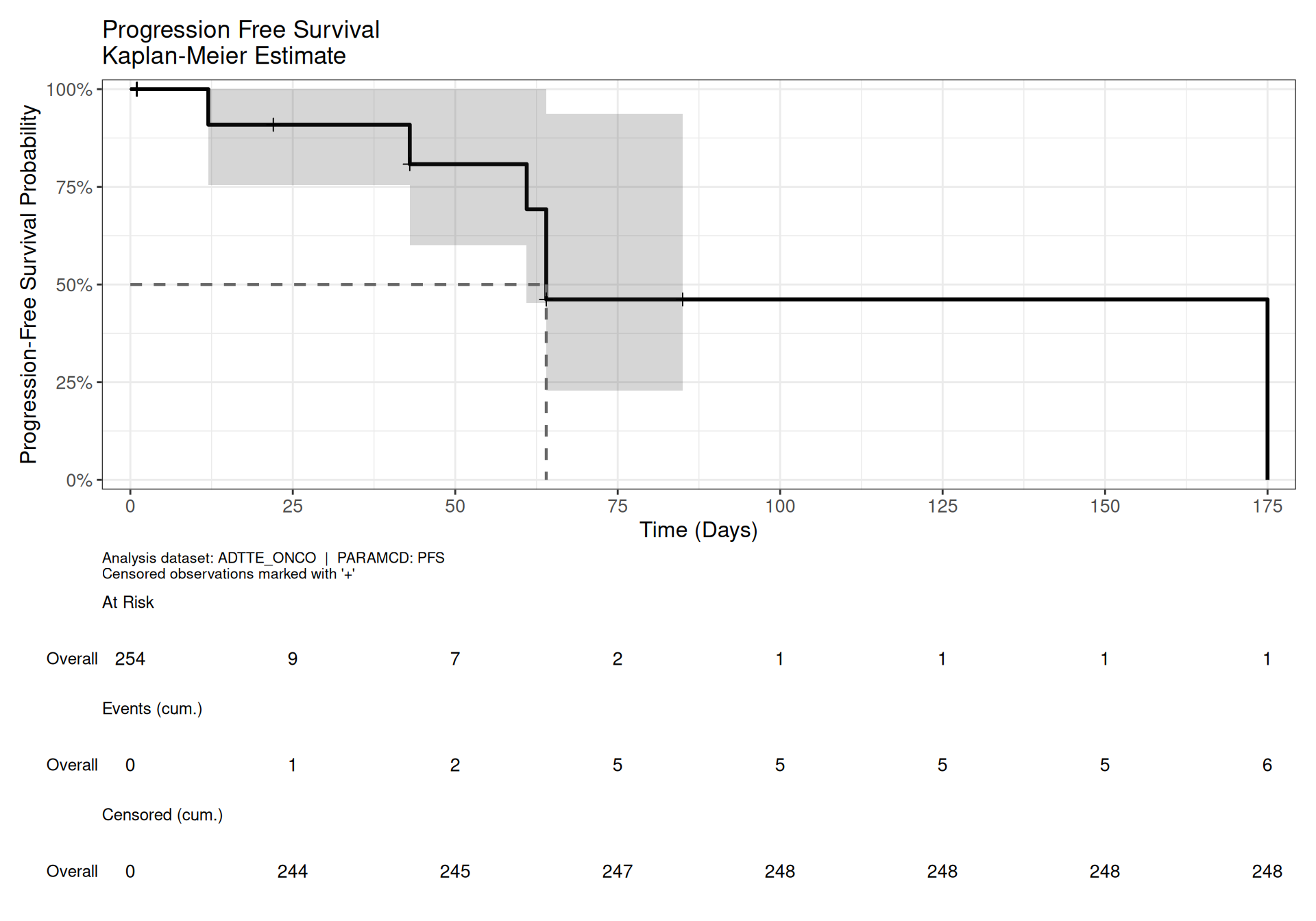
## Kaplan-Meier Plot
The plot below uses `survfit2()` with `Surv_CNSR()` to fit the survival model.
Because `PARAM` and `PARAMCD` are present in the data, `{ggsurvfit}`
automatically uses `PARAM` as the y-axis label — a key CDISC-aware feature.
The KM plot is shown once here and shared across all summary tables below.
```{r km-plot}
#| message: false
#| warning: false
#| fig-width: 10
#| fig-height: 7
# ── Fit the survival model ─────────────────────────────────────────────────────
# survfit2() is preferred over survfit() as it tracks the calling environment,
# enabling clean legend labels and p-value computation downstream.
km_fit <- survfit2(Surv_CNSR(AVAL, CNSR) ~ 1, data = adtte_pfs)

# ── Build the plot ─────────────────────────────────────────────────────────────
km_fit |>
  ggsurvfit(linewidth = 1) +
  # ── Explicit color scales prevent the site theme from stripping colour to B&W ─
  scale_color_manual(values = c("#2c7bb6")) +
  scale_fill_manual(values = c("#2c7bb6")) +
  add_confidence_interval() +
  add_risktable(
    risktable_stats = c("n.risk", "cum.event", "cum.censor"),
    risktable_group = "risktable_stats",
    stats_label = list(
      n.risk     = "At Risk",
      cum.event  = "Events (cum.)",
      cum.censor = "Censored (cum.)"
    ),
    theme = theme_risktable_default(axis.text.y.size = 9, plot.title.size = 9)
  ) +
  add_quantile(
    y_value   = 0.5, # median survival guideline
    color     = "gray40",
    linewidth = 0.75,
    linetype  = "dashed"
  ) +
  add_censor_mark(shape = 3, size = 2) +
  scale_ggsurvfit() +
  labs(
    title = paste0(unique(adtte_pfs$PARAM), "\nKaplan-Meier Estimate"),
    x = "Time (Days)",
    y = "Progression-Free Survival Probability",
    caption = paste0(
      "Analysis dataset: ADTTE_ONCO  |  PARAMCD: ", unique(adtte_pfs$PARAMCD),
      "\nCensored observations marked with '+'"
    )
  ) +
  theme_ggsurvfit_default() +
  theme(plot.caption = element_text(hjust = 0, size = 8))
```
**Figure notes:**
* The shaded band shows the pointwise 95% confidence interval (default:
log-log transformed).
* The dashed horizontal line marks the 50% survival probability; its
intersection with the curve gives the median survival time.
* `+` marks indicate individual censored observations.
* The risk table beneath the plot shows cumulative counts aligned to the
x-axis breaks.
---
## Summary Tables
`{gtsummary}`'s `tbl_survfit()` consumes the `km_fit` `survfit2` object directly
to produce publication-ready tables. The statistics are extracted and formatted
in a single pipeline.
### Median Survival Table
```{r median-table}
#| message: false
#| warning: false
# ── Median survival with 95% CI ────────────────────────────────────────────────
tbl_survfit(
  km_fit,
  probs        = 0.5, # 50th percentile = median
  label_header = "**Median (95% CI)**"
) |>
  modify_caption(
    paste0(
      "**Table 1. Median Progression-Free Survival**",
      "\nADTTE_ONCO  |  PARAMCD: ", unique(adtte_pfs$PARAMCD)
    )
  ) |>
  bold_labels()
```
### Survival Probability Table
This table shows estimated PFS probabilities at clinically meaningful time
points. Here we use 1, 2, 3, and 6 months (expressed in days, matching the
units of `AVAL` in `adtte_onco`). Adjust `times` to match the units in your dataset.
```{r prob-table}
#| message: false
#| warning: false
# ── Survival probability at selected time points ───────────────────────────────
# AVAL in adtte_onco is in days
tbl_survfit(
  km_fit,
  times        = c(30, 60, 90, 180), # 1, 2, 3, 6 months in days
  label_header = "**PFS Probability (95% CI)**"
) |>
  modify_header(
    label = "**Time Point**"
  ) |>
  modify_table_body(
    ~ .x |>
      mutate(label = recode(label,
        "30"  = "1 month",
        "60"  = "2 months",
        "90"  = "3 months",
        "180" = "6 months"
      ))
  ) |>
  modify_caption(
    paste0(
      "**Table 2. Progression-Free Survival Probability at Selected Time Points**",
      "\nADTTE_ONCO  |  PARAMCD: ", unique(adtte_pfs$PARAMCD)
    )
  ) |>
  bold_labels()
```
::: {.callout-note}
## ARD output
Every `{gtsummary}` table stores its underlying statistics in a `.$cards` slot
as an Analysis Results Data (ARD) object conforming to the emerging CDISC
Analysis Results Standard. You can also generate a standalone survival ARD for
audit, downstream rendering, or cross-validation using
`cardx::ard_survival_survfit()`:
```r
# Median survival ARD
adtte_pfs |>
  cardx::ard_survival_survfit(
    y     = "Surv_CNSR(AVAL, CNSR)",
    probs = 0.5
  )

# Time-point survival probability ARD
adtte_pfs |>
  cardx::ard_survival_survfit(
    y     = "Surv_CNSR(AVAL, CNSR)",
    times = c(30, 60, 90, 180) # days
  )
```
The `y` argument must be passed as a character string when using the data frame
method. See the [`{cardx}` documentation](https://insightsengineering.github.io/cardx/main/reference/ard_survival_survfit.html)
for full details.
:::
---
## Best Overall Response Table
The Best Overall Response (BOR) table is a standard oncology efficacy output
summarising each subject's best RECIST response category across all post-baseline
assessments. Using `PARAMCD == "CBOR"` (Confirmed Best Overall Response) aligns
with the primary regulatory definition of ORR as confirmed CR + PR.
The `{gtsummary}` `tbl_summary()` function produces the category counts and
percentages directly from `AVALC`. Response categories are ordered from best to
worst (CR → PR → SD → NON-CR/NON-PD → PD → NE → MISSING) using a factor.
The ORR (CR + PR) is then derived and reported separately in the inline chunk below.
```{r bor-setup}
#| message: false
#| warning: false
# ── Filter to CBOR parameter ──────────────────────────────────
# ANL01FL == "Y" restricts to the primary analysis flag records.
adrs_bor <- adrs_onco |>
  filter(PARAMCD == "CBOR" & ANL01FL == "Y") |>
  mutate(
    # Order AVALC from best to worst response for table display
    AVALC = fct_relevel(
      AVALC,
      "CR", "PR", "SD", "NON-CR/NON-PD", "PD", "NE", "MISSING"
    )
  )
```
```{r bor-table}
#| message: false
#| warning: false
# ── Best Overall Response table by treatment arm ───────────────────────────────
adrs_bor |>
  tbl_summary(
    by = ARM,
    include = AVALC,
    label = list(AVALC = "Best Overall Response"),
    statistic = list(AVALC = "{n} ({p}%)"),
    digits = list(AVALC = list(0, 1))
  ) |>
  add_overall(last = TRUE) |>
  add_n() |>
  bold_labels() |>
  modify_header(label = "**Response**") |>
  modify_caption(
    paste0(
      "**Table 3. Confirmed Best Overall Response (RECIST 1.1)**",
      "\nADRS_ONCO  |  PARAMCD: CBOR  |  ANL01FL = Y"
    )
  )
```
The ORR (overall response rate, CR + PR) is not directly produced by
`tbl_summary()` as a combined row, but can be derived and appended using
`tbl_stack()` or reported inline:
```{r orr-inline}
#| message: false
#| warning: false
# ── ORR: proportion with CR or PR, by arm ─────────────────────────────────────
adrs_bor |>
  summarise(
    .by    = ARM,
    n_resp = sum(AVALC %in% c("CR", "PR"), na.rm = TRUE),
    n_tot  = n(),
    orr    = round(100 * n_resp / n_tot, 1)
  ) |>
  mutate(label = paste0(n_resp, "/", n_tot, " (", orr, "%)")) |>
  select(ARM, ORR = label) |>
  knitr::kable(caption = "Overall Response Rate (CR + PR) by Arm")
```
---
## Key Package Notes
**`Surv_CNSR()` vs `Surv()`**
CDISC ADTTE datasets use `CNSR = 0` for events and `CNSR = 1` for censoring —
the opposite of `survival::Surv()`. Using `Surv_CNSR(AVAL, CNSR)` removes
this error-prone manual recoding step, and it works identically in both the
`survfit2()` call for plotting and the `ard_survival_survfit()` call for ARDs:
```{r cnsr-note}
#| output: true
# ✗  Error-prone: requires manual recoding of CNSR
head(survival::Surv(adtte_pfs$AVAL, 1 - adtte_pfs$CNSR), 8)
# ✓  Correct CDISC-aware approach — identical result, no manual recoding needed
head(ggsurvfit::Surv_CNSR(adtte_pfs$AVAL, adtte_pfs$CNSR), 8)
```
**`survfit2()` vs `survfit()`**
`survfit2()` tracks the calling environment, which enables `{ggsurvfit}` to
cleanly remove raw variable names (e.g. `CNSR=0`) from figure legends and to
compute p-values via `survfit2_p()`. For ADTTE data, it also reads `PARAM`/`PARAMCD`
automatically to populate axis labels. Use `survfit2()` for all plotting work.
**Switching endpoints**
All outputs above are driven by the `adtte_pfs` object. To switch
to OS or RSD, simply change the filter at the top of the Setup section:
```{r endpoint-note}
#| eval: false
# Overall Survival — expect few events; median may not be estimable
adtte_os <- adtte_onco |> filter(PARAMCD == "OS")

# Duration of Response — responders only; smaller N than OS/PFS
# Note: admiralonco uses PARAMCD = "RSD", not "DOR"
adtte_rsd <- adtte_onco |> filter(PARAMCD == "RSD")
```
**Extending to multiple strata**
Because `adtte_onco` already contains `ARM` and `ARMCD` from the `{admiralonco}`
template, no ADSL join is needed to produce a stratified KM plot:
```{r strata-note}
#| eval: false
# With two arms (ARM), add_pvalue() computes and annotates a log-rank test p-value.
# Not applicable for single-arm fits (~ 1) — only add when comparing groups.
survfit2(Surv_CNSR(AVAL, CNSR) ~ ARM, data = adtte_pfs) |>
  ggsurvfit(linewidth = 1) +
  scale_color_brewer(palette = "Dark2") +
  scale_fill_brewer(palette = "Dark2") +
  add_confidence_interval() +
  add_risktable(
    theme = theme_risktable_default(axis.text.y.size = 9, plot.title.size = 9)
  ) +
  add_pvalue(location = "annotation") +
  scale_ggsurvfit()
```
---
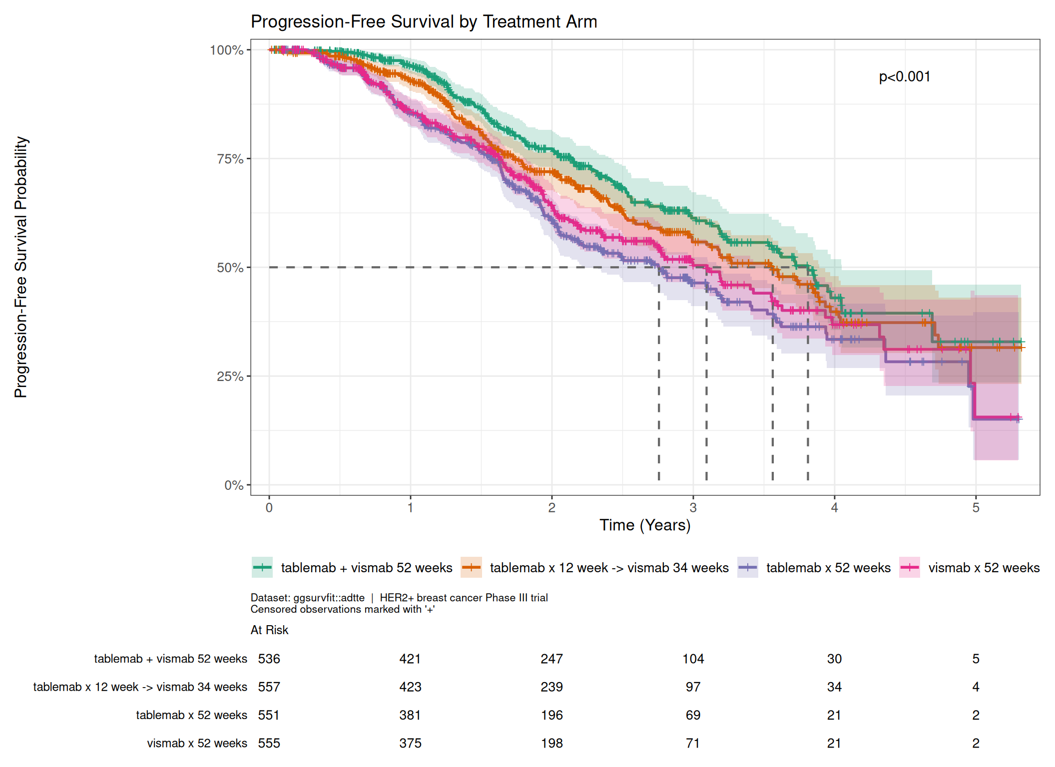
## Stratified KM Plot: `ggsurvfit::adtte`
`{ggsurvfit}` ships its own example ADTTE dataset — a four-arm Phase III breast
cancer trial (2,199 subjects, PFS endpoint, ~34% event rate) originally from the
[VIS-SIG Wonderful Wednesdays](https://github.com/VIS-SIG/Wonderful-Wednesdays/tree/master/data/2020/2020-04-08)
initiative. It provides a richer illustrative dataset than `adtte_onco` for
showing a **stratified KM plot**, since it has four well-separated treatment arms
with a good event rate and an estimable median.
The treatment variable is `TRT01P` (planned treatment at randomisation), which
contains the four arm labels directly. `STR01` is hormone receptor status — a
stratification covariate, not the treatment assignment.
```{r km-plot-adtte}
#| message: false
#| warning: false
#| fig-width: 11
#| fig-height: 8
# ── ggsurvfit::adtte — four-arm breast cancer PFS trial ────────────────────────
# TRT01P = planned treatment; STR01 = hormone receptor status (not treatment)
survfit2(Surv_CNSR(AVAL, CNSR) ~ TRT01P, data = ggsurvfit::adtte) |>
  ggsurvfit(linewidth = 1) +
  scale_color_brewer(palette = "Dark2") +
  scale_fill_brewer(palette = "Dark2") +
  add_confidence_interval() +
  add_risktable(
    risktable_stats = "n.risk",
    stats_label = list(n.risk = "At Risk"),
    theme = theme_risktable_default(axis.text.y.size = 9, plot.title.size = 9)
  ) +
  add_quantile(
    y_value   = 0.5,
    color     = "gray40",
    linewidth = 0.75,
    linetype  = "dashed"
  ) +
  add_censor_mark(shape = 3, size = 1.5) +
  add_pvalue(location = "annotation", x = 4.5) +
  scale_ggsurvfit() +
  labs(
    title = "Progression-Free Survival by Treatment Arm",
    x = "Time (Years)", # ggsurvfit::adtte AVAL is in years
    y = "Progression-Free Survival Probability",
    caption = paste0(
      "Dataset: ggsurvfit::adtte  |  HER2+ breast cancer Phase III trial",
      "\nCensored observations marked with '+'"
    )
  ) +
  theme_ggsurvfit_default() +
  theme(
    plot.caption  = element_text(hjust = 0, size = 8),
    legend.title  = element_blank()
  )
```
**Figure notes:**
* The risk table shows only `n.risk` here (rather than cumulative events and
censored) to keep the four-strata table readable at standard figure width.
* The p-value is an **overall log-rank test** comparing survival across all four
arms simultaneously. It is placed as an annotation (rather than in the caption)
to remain visible when the figure is used standalone. For pairwise comparisons
of each active arm vs. a reference, a Cox model or `survdiff()` with specific
contrast coding would be needed instead.
* `ggsurvfit::adtte` contains only a single PFS endpoint per subject, so no
`filter(PARAMCD == ...)` step is needed.
---
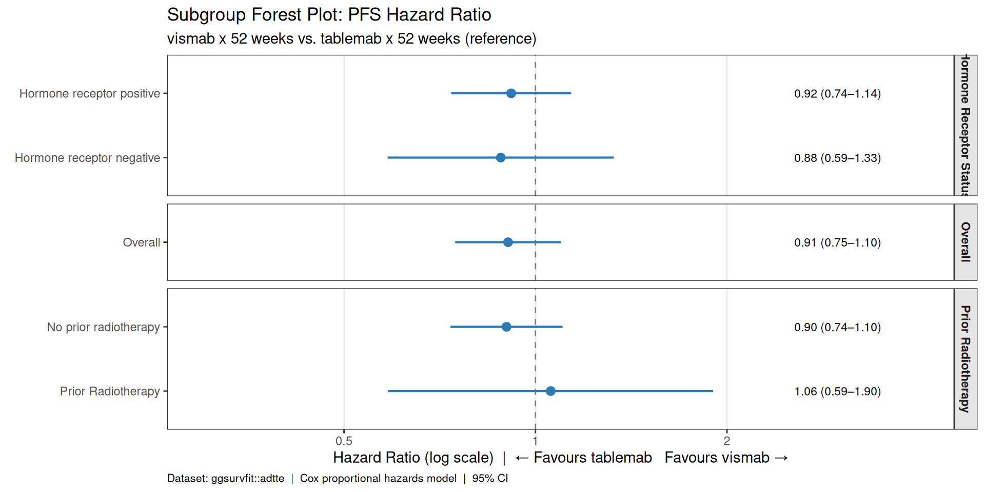
## Subgroup Forest Plot
A subgroup forest plot displays the hazard ratio (HR) and 95% confidence interval
from a Cox model for each subgroup level, giving a visual summary of whether the
treatment effect is consistent across key patient characteristics.
Here we restrict `ggsurvfit::adtte` to two arms — `tablemab x 52 weeks`
(reference) and `vismab x 52 weeks` (active) — and fit separate Cox models
within each level of `STR01L` (hormone receptor status) and `STR02L`
(prior radiotherapy), plus an overall row.
```{r forest-setup}
#| message: false
#| warning: false
# ── Restrict to two arms ───────────────────────────────────────────────────────
adtte_2arm <- ggsurvfit::adtte |>
  filter(TRT01PN %in% c(1, 2)) |>
  mutate(TRT01P = factor(TRT01P,
    levels = c("tablemab x 52 weeks", "vismab x 52 weeks")
  ))

# ── Helper: fit Cox and return a one-row HR summary ──────────────────────────
cox_hr <- function(data, subgroup, level) {
  fit <- coxph(Surv_CNSR(AVAL, CNSR) ~ TRT01P, data = data)
  tidy(fit, exponentiate = TRUE, conf.int = TRUE) |>
    mutate(
      subgroup = subgroup,
      level    = level,
      n        = nrow(data),
      n_events = sum(data$CNSR == 0)
    )
}

# ── Build rows: Overall + by STR01L + by STR02L ───────────────────────────────
str01_rows <- lapply(unique(adtte_2arm$STR01L), function(lv) {
  cox_hr(filter(adtte_2arm, STR01L == lv), "Hormone Receptor Status", lv)
})

str02_rows <- lapply(unique(adtte_2arm$STR02L), function(lv) {
  cox_hr(filter(adtte_2arm, STR02L == lv), "Prior Radiotherapy", lv)
})

forest_data <- bind_rows(
  cox_hr(adtte_2arm, "Overall", "Overall"),
  bind_rows(str01_rows),
  bind_rows(str02_rows)
) |>
  mutate(
    label = ifelse(level == "Overall", "Overall", paste0("  ", level)),
    label = factor(label, levels = rev(unique(label))),
    hr_label = sprintf("%.2f (%.2f\u2013%.2f)", estimate, conf.low, conf.high)
  )
```
```{r forest-plot}
#| message: false
#| warning: false
#| fig-width: 10
#| fig-height: 5
ggplot(forest_data, aes(x = estimate, y = label)) +
  geom_vline(xintercept = 1, linetype = "dashed", color = "gray50") +
  geom_pointrange(
    aes(xmin = conf.low, xmax = conf.high),
    color = "#2c7bb6",
    linewidth = 0.75,
    fatten = 4
  ) +
  geom_text(
    aes(x = 3.5, label = hr_label),
    hjust = 1, size = 3
  ) +
  scale_x_log10(
    limits = c(0.3, 4),
    breaks = c(0.5, 1, 2),
    labels = c("0.5", "1", "2")
  ) +
  facet_grid(subgroup ~ ., scales = "free_y", space = "free") +
  labs(
    title    = "Subgroup Forest Plot: PFS Hazard Ratio",
    subtitle = "vismab x 52 weeks vs. tablemab x 52 weeks (reference)",
    x        = "Hazard Ratio (log scale)  |  \u2190 Favours tablemab   Favours vismab \u2192",
    y        = NULL,
    caption  = "Dataset: ggsurvfit::adtte  |  Cox proportional hazards model  |  95% CI"
  ) +
  theme_bw() +
  theme(
    strip.background    = element_rect(fill = "gray90"),
    strip.text          = element_text(face = "bold"),
    panel.grid.minor    = element_blank(),
    panel.grid.major.y  = element_blank(),
    plot.caption        = element_text(hjust = 0, size = 8)
  )
```
**Figure notes:**
* HR < 1 favours `tablemab` (reference arm); HR > 1 favours `vismab`.
* The dashed vertical line at HR = 1 represents no treatment difference.
* Confidence intervals that cross 1 indicate no statistically significant
difference in that subgroup at the 5% level.
* This is for illustration only — the dataset uses anonymised arm names and
should not be interpreted as a real-world efficacy comparison.
---
## Customization Tips
You can easily tailor the appearance and output of your tables and plots:
- **Themes & Colors:**
- Use `theme_ggsurvfit_default()` or any `ggplot2` theme (e.g., `theme_minimal()`, `theme_bw()`) to change the look of plots.
- Adjust color palettes with `scale_color_manual()`, `scale_fill_brewer()`, or your own color vectors.
- **Fonts & Labels:**
- Modify axis titles, legend text, and captions using `labs()` and `theme()` arguments (e.g., `axis.title = element_text(size = 14)`).
- **Exporting:**
- Save plots with `ggsave("plot.png", width = 8, height = 6)`.
- Export tables to Word/HTML with `as_flextable()` or `as_gt()` from `{gtsummary}`.
- **Table Formatting:**
- Use `{gtsummary}` functions like `bold_labels()`, `modify_caption()`, and `modify_header()` for custom table styling.
See the documentation for each package for more advanced customization options.